Citizen Science Approach
We are using a citizen science based approach to understand how humans and coyotes are interacting in Edmonton (Figure 4). Citizen science is the engagement of the general public in the scientific process by enabling the public collection and sharing of data to increase scientific knowledge. Successful citizen science projects include: the Audubon Society’s Christmas Bird Count to record over-wintering species; the Alberta Plant Watch program to track bloom dates; and iNaturalist, which helps track global biodiversity.

Figure 4. A visual representation of the citizen science based approach used in this study.
Report Collection

|
Since 2010, we have encouraged the public to report coyote sightings and encounters on the Edmonton Urban Coyote Project website (www.edmontonurbancoyotes.ca/reportsighting.php), gathering a large database of citizen reports.
When submitting a report citizens can indicate the time and date of the report, the location by placing a pin on google maps, the type of report and have the option to add additional comments. The type of report is either: A) a sighting at a distance with no perceived interaction or B) an encounter, a perceived interaction at close range. Between January 2011 and December 2019, 7,556 reports were made by 6,953 different people. We excluded all reports from the year 2011 because the website had yet to gain popularity and reporting was low (N=112). These reports were analyzed using R software (R Core Team 2019) and ArcGIS 10.7.1 (Esri 2019). |
Study Area
Edmonton, Alberta is a large northern city with a population of over 800,000 and an area of 684 square kilometres. A large river valley and park system transects Edmonton, providing habitat and connectivity to various species including coyotes and many of their natural prey items (Murray et al. 2015a). Across the city, there are various types of coyote habitats in which reports occur (Figure 5, Table 1). Because of recent land annexations, the city limits technically extend farther north-east and south-west than shown on Figure 5, but because these areas consist of sparsely-populated agricultural land they were removed from the analyses.

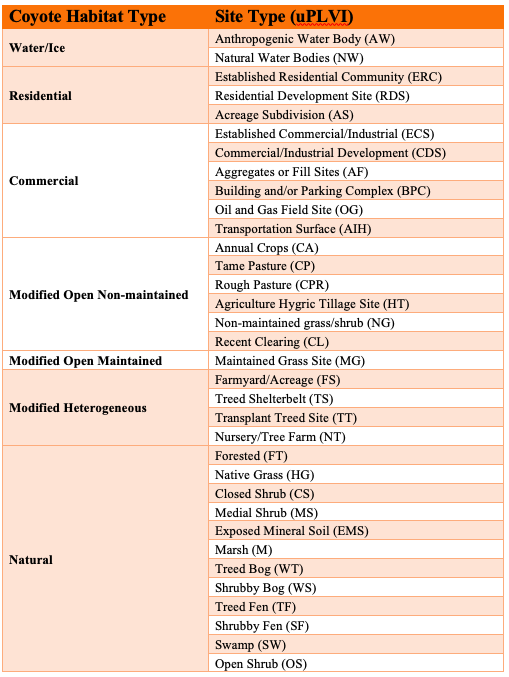
Figure 5. Coyote habitat distribution across Edmonton, using data from the City of Edmonton uPLVI (Urban Primary Land and Vegetation Inventory) land cover data (City of Edmonton, 2018). Land cover classes were categorized into different coyote habitat types based on anthropogenic influence and vegetation cover (Table 1).
|
Table 1. Coyote habitat types in Figure 5 were categorized by combining site types from the City of Edmonton uPLVI (Urban Primary Land and Vegetation Inventory) land cover data (City of Edmonton, 2018).
|
Statistical Analysis
To determine if coyote reports occurred in specific habitat types, I calculated the density of sightings and encounters per square kilometre based on the spatial intersection of reports and habitat types (tabulate intersection function in ArcGIS). I used a chi square test of independence to determine if the count of sightings and encounters in habitat types differed from the expected count. The expected count in each habitat type was calculated based on the total number of sightings or encounters multiplied by the proportion of total area made up by that habitat type.
I used a chi square test of independence followed by pairwise comparisons to determine if the number of sightings and encounters across seasons (breeding, pup-rearing and dispersal) and a diel scale (six hour time intervals) were significantly different. I adjusted all pairwise comparison P-values for multiple comparisons with the Bonferroni-Holm correction.
To determine if encounters have increased between 2012 and 2019, I calculated a conflict score for each month by standardizing the number of encounters by the number of sightings for that month (encounters/sightings). Conflict scores were plotted over time to allow for the visualization of trends, and the smoothed mean was calculated using the stat_smooth function in R. Confidence bounds (95%) were computed using the loess method, which uses a t-based approximation to determine the upper and lower bounds.
